Testing the Central Limit Theorem

In my first post ever, I would like to illustrate the central limit theorem, which pinpoints the importance of Normal distribution. I took the main idea from Statistics in a Nutshell, 2nd edition, chapter 3.

Background

Central Limit Theorem (CLT) establishes that in many situations, “when independent random variables are added, their properly normalized sum tends toward a normal distribution” (Wikipedia). It means that, if $X_1,\ldots,X_n$ is a random sample drawn from a distribution with mean $\mu$ and variance $\sigma^2$, then

where $\bar{X}$ is the sample mean. Interestingly, CLT doesn’t specify an underlying distribution!

Simulations

The approach we’ll be taking here is to draw random values from uniform, lognormal and inverse gamma distributions, calculate their means and then compare them with the theoretical value given by the CLT. For this, we are going to use NumPy, seaborn, and scipy.stats modules

import numpy as np
import matplotlib.pyplot as plt
import seaborn as sns
from scipy.stats import norm, uniform, lognorm, invgamma

seed = 12345 # Fix the random seed to guarantee reproducibility
rng = np.random.default_rng(seed)

Normal distribution

scipy.stats gives access to a variety of probability distributions. They are parametrized by location $L$ and scale $S$ parameters, and occasionally by a shape $s$ (https://docs.scipy.org/doc/scipy/reference/tutorial/stats/continuous.html). For instance, the normal distribution has a probability density function

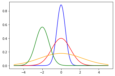
So, in this case, $L=\mu$ and $S=\sigma$ for the usual parametrization of normal distribution. Besides, we can instantiate different normal distributions with different $L$ and $S$ parameters. So, for reproducing this, we can instantiate 4 different distributions:

norm_L0S02 = norm(loc=0,scale=np.sqrt(0.2)) # $\mu=0,\sigma^2=0.2$ 
norm_L0S10 = norm(loc=0,scale=np.sqrt(1.0)) # $\mu=0,\sigma^2=0.2$ 
norm_L0S50 = norm(loc=0,scale=np.sqrt(5.0)) # $\mu=0,\sigma^2=5.0$ 
norm_Ln2S05 = norm(loc=-2,scale=np.sqrt(0.5)) # $\mu=-2,\sigma^2=0.5$ 

x = np.linspace(-5,5,100)
y_1 = norm_L0S02.pdf(x)
y_2 = norm_L0S10.pdf(x)
y_3 = norm_L0S50.pdf(x)
y_4 = norm_Ln2S05.pdf(x)

sns.lineplot(x=x,y=y_1,color='blue');
sns.lineplot(x=x,y=y_2,color='red');
sns.lineplot(x=x,y=y_3,color='orange');
sns.lineplot(x=x,y=y_4,color='green');

Unifrom Distribution

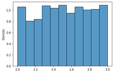
FFirst, we create a uniform distribution $U(2,3)$

uniform_23 = uniform(loc=2,scale=1)

A unifrom distribution looks like this:

sns.histplot(uniform_23.rvs(1000),stat='density');

Again, scipy.stats provides a convenient way to extract the mean and variance of a distribution

u_23_mean, u_23_var = uniform_23.stats(moments='mv')
print("Mean: {:0.2f}, Variance: {:0.3f}".format(u_23_mean,u_23_var))

Mean: 2.50, Variance: 0.083

Ok, so far, so good. Next, let’s take 1000 samples of size $n = 10$ and calculate their means. Function rvs draws random values from a given distribution:

uni_means = [uniform_23.rvs(size=10).mean() for x in range(1000)]

sns.histplot(uni_means,stat='density');

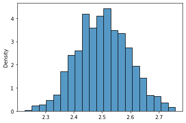
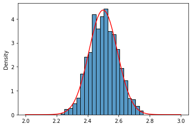
Well, that really looks like a normal distribution of $\mu = 2.5$ and $\frac{\sigma^2}{n} = 0.0083$, right?. Let’s do a visual inspection using the Probability Density Function (pdf) of a normal distribution (better safe than sorry)

norm_uni = norm(loc=u_23_mean,scale=np.sqrt(u_23_var/10))
x = np.linspace(2,3,100) 

sns.histplot(uni_means,stat='density');
sns.lineplot(x=x,y=norm_uni.pdf(x),color='red');

Lognormal Distribution

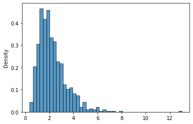
Ok, but uniform distribution is kind of a “classic,” right? What about a less known distribution?. We are going to try with the lognormal distribution.

lnr_05_2 = lognorm(s=1/2,scale=2)

This distribution looks like this:

sns.histplot(lnr_05_2.rvs(1000),stat='density');

Again, we retrieve the parameters from the distribution:

lnr_05_2_mean, lnr_05_2_var = lnr_05_2.stats(moments='mv')
print("Mean: {:0.2f}, Variance: {:0.3f}".format(lnr_05_2_mean,lnr_05_2_var))

Mean: 2.27, Variance: 1.459

As in the previous example, let’s take 1000 samples of size 10 and calculate their means

lnr_means_10 = [lnr_05_2.rvs(size=10).mean() for x in range(1000)]

sns.histplot(lnr_means_10,stat='density');

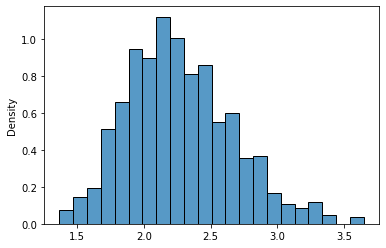
Hmmm… Now it doesn’t look very normal, isn’t it?. Let’s see

norm_lnr = norm(loc=lnr_05_2_mean,scale=np.sqrt(lnr_05_2_var/10))
x = np.linspace(0.5,4.5,100)

sns.histplot(lnr_means_10,stat='density');
sns.lineplot(x=x,y=norm_lnr.pdf(x),color='red');

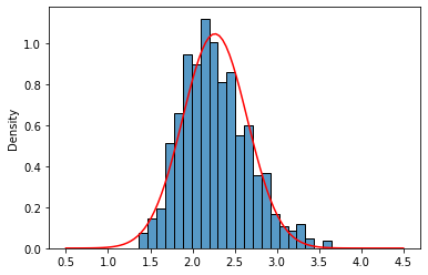
It kinds of fits but is not very convincing. The tails seem a little bit off. CLT is valid for $n \rightarrow \infty$, so there is no fixed n that works for every distribution. Let’s be bold and check with $n$=100

lnr_means_100 = [lnr_05_2.rvs(size=100).mean().mean() for x in range(1000)]
sns.histplot(lnr_means_100,stat='density');
norm_lnr = norm(loc=lnr_05_2_mean,scale=np.sqrt(lnr_05_2_var/100))
x = np.linspace(1.5,3,100) #norm.ppf: Percent point function (inverse of `cdf`)
sns.lineplot(x=x,y=norm_lnr.pdf(x),color='red');

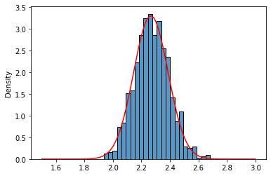
More likely, isn’t it?

Inverse Gamma

Let’s try the last distribution, an inverse gamma. It takes an $a$ parameter:

invgamma_407 = invgamma(a=4.07)

sns.histplot(invgamma_407.rvs(1000),stat='density');

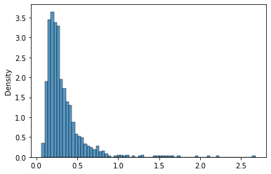
As before, let’s recover the parameters:

invgamma_407_mean, invgamma_407_var = invgamma_407.stats(moments='mv')
print("Mean: {:0.2f}, Variance: {:0.3f}".format(invgamma_407_mean,invgamma_407_var))

Mean: 0.33, Variance: 0.051

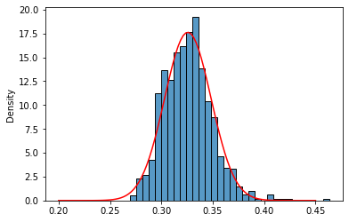
And generate the histograms of 100 and 1000 samples means with their respective normal estimations:

invgamma_means_0100 = [invgamma_407.rvs(size= 100).mean() for x in range(1000)]
invgamma_means_1000 = [invgamma_407.rvs(size=1000).mean() for x in range(1000)]

sns.histplot(invgamma_means_0100,stat='density');
norm_invg_1 = norm(loc=invgamma_407_mean,scale=np.sqrt(invgamma_407_var/100))
x = np.linspace(0.2,0.45,100)
sns.lineplot(x=x,y=norm_invg_1.pdf(x),color='red');

sns.histplot(invgamma_means_1000,stat='density');
norm_invg_2 = norm(loc=invgamma_407_mean,scale=np.sqrt(invgamma_407_var/1000))
x = np.linspace(0.25,0.40,100) #norm.ppf: Percent point function (inverse of `cdf`)
sns.lineplot(x=x,y=norm_invg_2.pdf(x),color='red');

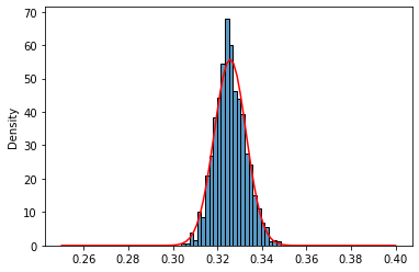
Again, as for the lognormal distribution, for $n=100$ normal approximation seems a little bit off in the tails, probably because of the skewed shape of inverse gamma distribution.

And that’s it! CLT is a useful tool from both theoretical and practical perspectives because it allows us to model the mean of any distribution for (sufficiently) large samples.